

tracage de points entre deux variables numériques (+ color(cat1) +facet_wrap(cat3))
24 déc. 2018geom_point :tracage des points entre deux variables numérique
ggplot(data = diamonds) +
aes(x = carat, y = price, color = clarity) +
geom_point() +
theme_minimal()

color=variable catégorielle :tracage des points entre deux variables numérique avec couleur par rapport à une variable catégorielle
ggplot(data = diamonds) +
aes(x = carat, y = price, color = clarity) +
geom_point() +
theme_minimal()

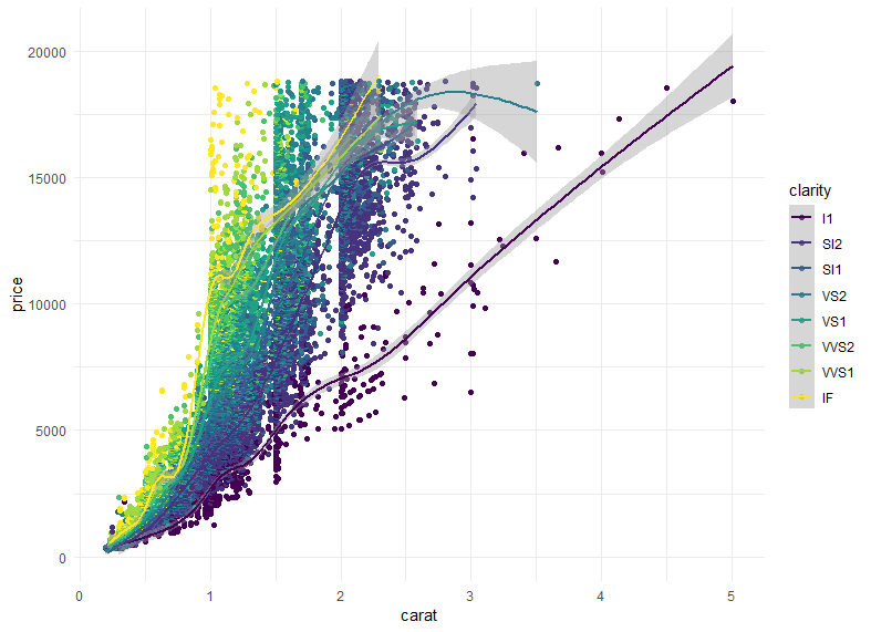
geom_smooth(): rajoute les lignes de la regression lineraire
ggplot(data = diamonds) +
aes(x = carat, y = price, color = clarity) +
geom_point() +
theme_minimal() +
geom_smooth()
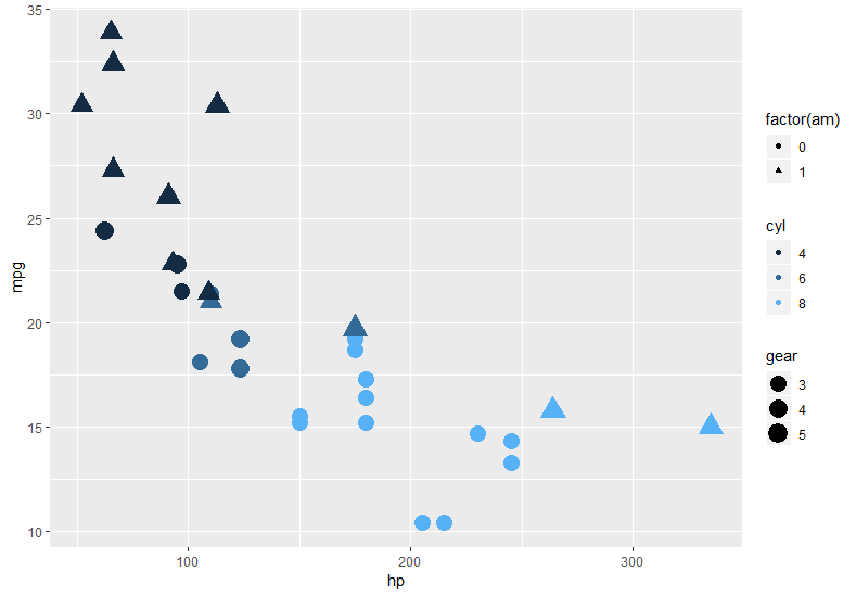
courbes en rajouter 3 catégories avec grosseurs de points différents
ggplot(data = mtcars, aes(
  x = hp, y = mpg,
  size = gear, color = cyl,
  shape = factor(am)
)) +
  geom_point() +
  scale_size_continuous(
    breaks = c(3, 4, 5),
    limits = c(0, 5)
  ) +
  scale_color_continuous(breaks = c(4, 6, 8)) +
  guides(color = guide_legend())
facet_wrap(vars(color)):permet de rajouter des cadrants(n catégories) par rapport à la catégorie
ggplot(data = diamonds) +
aes(x = carat, y = price, color = clarity) +
geom_point() +
theme_minimal() +
geom_smooth() +
facet_wrap(vars(color))

Rajout d'options avec guides et coord_fixed
> head(data)
V1 V2 Col
1 6.002504 0.03150495 320
2 6.004021 0.06316767 538
3 6.004545 0.09495748 1731
4 6.004069 0.12684338 1676
5 6.002587 0.15879411 174
6 6.000094 0.19077814 1955
ggplot(data,aes(x = V1, y = V2, color = Col)) +
geom_point(size = 2) + guides(color = FALSE) +
coord_fixed()

autres visualisations:
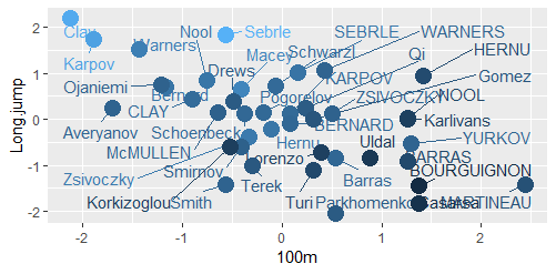
1/
decathlonR <- decathlon
decathlonR[1:10] <- scale(decathlonR[1:10])
decathlonR2 <- decathlonR %>% rownames_to_column()
ggplot(data= decathlonR2, aes(x = `100m`,
y = Long.jump,
color = Points)) +
geom_text_repel(aes(label = rowname),
box.padding = unit(0.75, "lines")) +
geom_point(size = 5) +
guides(color = FALSE)
2/
TemperatureMDS <- cmdscale(DistTemperature)
head(TemperatureMDS)
[,1] [,2]
Amsterdam 0.5444069 1.23241284
Athens -6.1934962 -0.94443738
Berlin 1.0036551 -0.03157218
Brussels 0.1724224 1.05070563
Budapest -0.7865432 -1.58932143
Copenhagen 2.0677061 0.41386030
ggplot(data = data.frame(X1 = TemperatureMDS[,1], X2 = TemperatureMDS[,2]), aes(x = X1, y = X2)) +
geom_point() + geom_text_repel(label = row.names(temperature))


/https%3A%2F%2Fassets.over-blog.com%2Ft%2Fcedistic%2Fcamera.png)
/http%3A%2F%2Fassets.over-blog.com%2Ft%2Ffloating_posts%2Fimages%2Fcover.jpg)